Path Signatures for Handwritten Digit Classification Using Esig
This notebook is based upon the use of path signature techniques to tackle the task of recognising handwritten numerical digits. The dataset considered is the MNIST sequence data (https://edwin-de-jong.github.io/blog/mnist-sequence-data/) corresponding to the MNIST handwritten digit data set by Edwin D.De Jong.
The task we consider is sequence classification; given a sequence of pen strokes (i.e. pen locations with additional information about the stroke at each given pen location), we aim to predict the digit it represents. As an alternative approach, we disregard information about pen strokes and consider simply the sequence of pen locations. The MNIST sequence dataset is labelled, thus we will initially explore supervised learning approaches. In addition, the notebook explores semi-supervised and unsupervised approaches based upon clustering.
To compute the path signature features for training our models, we use esig.
Set up the Notebook
We begin by setting up the coding environment.
Install Dependencies
The following cell is only required to be executed if any of the listed packages are not already installed.
import sys
!{sys.executable} -m pip install -r requirements.txt
Import Packages
import joblib
from joblib import Parallel, delayed
import os.path
import pickle
import tarfile
import urllib.request

import esig
import matplotlib.pyplot as plt
import numpy as np

import MNIST_funcs
The module ‘MNIST_funcs’ is a collection of documented functions, written for the task of applying path signature techniques to the MNIST sequence classification task.
Download the Dataset
The MNIST sequence dataset is stored in a compressed tarfile format with the extension tar.gz . We first download this compressed tarfile, before opening it and extracting its contents to a directory named ‘mnist_data’ below the current working directory.
MNIST_DOWNLOAD_URL = \
    'https://raw.githubusercontent.com/edwin-de-jong/mnist-digits-stroke-sequence-data/master/sequences.tar.gz'

TARGET_FILE = 'sequences.tar.gz'
DATA_DIRECTORY = 'mnist_data'

if not os.path.exists(DATA_DIRECTORY):

    print('Downloading data...')
    urllib.request.urlretrieve(MNIST_DOWNLOAD_URL, TARGET_FILE)

    print('Extracting data...')
    tar = tarfile.open(TARGET_FILE)
    tar.extractall(DATA_DIRECTORY)
    tar.close()
Extract Sequences
We next extract the pen-stroke sequences, the location sequences and the labels contained in the ‘mnist_data’ directory. The contents are pre-split into \(60\,000\) training instances and \(10\,000\) testing instances. We carry out the extraction using the ‘mnist_train_data’ and ‘mnist_test_data’ functions from the ‘MNIST_funcs’ package, which are documented as follows:
help(MNIST_funcs.mnist_train_data)
Help on function mnist_train_data in module MNIST_funcs:

mnist_train_data(data_directory, cpu_number)
    Read the training data from the specified directory.

    Returns three lists; the first is a list of the streams formed by the 2D
    points data, the second is a list of streams of the 3D input data recording
    in the first two entries the change in x and y coordinates from the previous
    point and when the pen leaves the paper in the third entry. The fourth
    coordinate used to indicate when one figure ends and the next begins is
    ignored in this extraction. See the MNIST sequences project website for full
    details. The third returned list is a list of integer labels marking the
    number corresponding to each sequence.
help(MNIST_funcs.mnist_test_data)
Help on function mnist_test_data in module MNIST_funcs:

mnist_test_data(data_directory, cpu_number)
    Read the training data from the specified directory.

    Returns three lists; the first is a list of the streams formed by the 2D
    points data, the second is a list of streams of the 3D input data recording
    in the first two entries the change in x and y coordinates from the previous
    point and when the pen leaves the paper in the third entry. The fourth
    coordinate used to indicate when one figure ends and the next begins is
    ignored in this extraction. See the MNIST sequences project website for full
    details. The third returned list is the integer labels marking the number
    corresponding to each sequence.
N_CPU = joblib.cpu_count()
train_points, train_inputs, train_targets = MNIST_funcs.mnist_train_data(DATA_DIRECTORY, N_CPU)
test_points, test_inputs, test_targets = MNIST_funcs.mnist_test_data(DATA_DIRECTORY, N_CPU)
We use used every available CPU for parallelisation. Depending on your hardware this may not be the best option, and you might prefer to change ‘N_CPU’ to a more suitable choice.
With the sequences and labels extracted, we will examine an example sequence:
train_points[2], train_inputs[2], train_targets[2]
(array([[ 5.,  9.],
        [ 5., 10.],
        [ 5., 11.],
        [ 5., 12.],
        [ 5., 13.],
        [ 4., 14.],
        [ 4., 15.],
        [ 5., 16.],
        [ 6., 16.],
        [ 7., 16.],
        [ 8., 16.],
        [ 9., 16.],
        [10., 16.],
        [11., 16.],
        [12., 16.],
        [13., 16.],
        [14., 15.],
        [15., 15.],
        [16., 15.],
        [17., 15.],
        [18., 15.],
        [19., 15.],
        [19., 16.],
        [19., 17.],
        [19., 18.],
        [18., 19.],
        [18., 20.],
        [18., 21.],
        [18., 22.],
        [18., 23.],
        [-1., -1.],
        [19., 14.],
        [20., 13.],
        [20., 12.],
        [20., 11.],
        [21., 10.],
        [21.,  9.],
        [22.,  8.],
        [22.,  7.],
        [22.,  6.]]),
 array([[ 5.,  9.,  0.],
        [ 0.,  1.,  0.],
        [ 0.,  1.,  0.],
        [ 0.,  1.,  0.],
        [ 0.,  1.,  0.],
        [-1.,  1.,  0.],
        [ 0.,  1.,  0.],
        [ 1.,  1.,  0.],
        [ 1.,  0.,  0.],
        [ 1.,  0.,  0.],
        [ 1.,  0.,  0.],
        [ 1.,  0.,  0.],
        [ 1.,  0.,  0.],
        [ 1.,  0.,  0.],
        [ 1.,  0.,  0.],
        [ 1.,  0.,  0.],
        [ 1., -1.,  0.],
        [ 1.,  0.,  0.],
        [ 1.,  0.,  0.],
        [ 1.,  0.,  0.],
        [ 1.,  0.,  0.],
        [ 1.,  0.,  0.],
        [ 0.,  1.,  0.],
        [ 0.,  1.,  0.],
        [ 0.,  1.,  0.],
        [-1.,  1.,  0.],
        [ 0.,  1.,  0.],
        [ 0.,  1.,  0.],
        [ 0.,  1.,  0.],
        [ 0.,  1.,  0.],
        [ 0.,  0.,  1.],
        [ 1., -9.,  0.],
        [ 1., -1.,  0.],
        [ 0., -1.,  0.],
        [ 0., -1.,  0.],
        [ 1., -1.,  0.],
        [ 0., -1.,  0.],
        [ 1., -1.,  0.],
        [ 0., -1.,  0.],
        [ 0., -1.,  0.]]),
 4)
The first array captures the locations of the pen tip as the digit is drawn, the second array captures the same information in its first two columns (interpreted as horizontal and vertical changes from the previous location) whilst its third column records the number of strokes (the presence of a \(1\) indicates a stroke ending; so the digit in this example is drawn via two separate strokes) and the third returned value is the sequences label telling us that this sequence corresponds to a \(4\).
Path Signature Methodology
The classification problem that we consider consists of learning how to use either of the two sequences to accurately predict the label. The piecewise linear interpolation of the sequence of locations forms a continuous path in \(\mathbb{R}^2\), and the piecewise linear interpolation of the sequence of pen strokes forms a continuous path in \(\mathbb{R}^3\). The challenge involves understanding the effect of these paths.
The Path Signature
The path signature is a central object in the mathematical field of rough path theory. It efficiently summarises paths such as the ones examined above in an essentially unique manner. The path signature is independent of the path’s time parameterisation, yet it still preserves the order in which events happen. The invariance to sampling rate is desirable, since the digit drawn is invariant to the speed at which it was drawn; a figure \(3\) is a figure \(3\) regardless of how quickly it is drawn. Moreover, this invariance ensures that the differing lengths of sequences is not an issue.
In mathematical terms, the signature of a path \(\gamma : [0,1] \to \mathbb{R}^d\) is the response of the exponential nonlinear system to the path. That is, the signature \(S(\gamma)\) is the solution to the universal differential equation
living in the tensor algebra \(T \left( \mathbb{R}^d \right)\). For the piecewise linear paths obtained via interpolation of the sequences of locations and pen strokes, the signature can be expressed in terms of iterated integrals of the paths. Namely, if \(\gamma : [0,1] \to \mathbb{R}^d\) is piecewise linear, then its signature is given by
where
By linearity, for each \(n \geq 1\) we have
for the standard orthonormal basis \(e_1 , \ldots , e_d \in \mathbb{R}^d\) and where each of the \(n\) integrations is along one coordinate axis. Hence the level \(n\) term of the signature \(S^n_{0,t}(\gamma)\) contains the collection of real numbers
for every possible choice of indices \(i_1 , \ldots , i_n \in \{1, \ldots , d\}\). There are \(d^n\) such choices, illustrating that the number of terms in the signature at level \(n\) grows exponentially with \(n\).
Making practical use of signatures requires overcoming the issue that the full signature is an infinite sequence of iterated integrals. We follow the most common solution of choosing a finite truncation level \(N \in \mathbb{N}\), and considering the truncated signature
i.e. only considering the iterated integrals of the path up to level \(N\). The exponential growth of the number of integrals in each new level mean it is common to only consider low-level (\(N \leq 10\)) truncations.
More details about the path signature may be found, for example, in any of the following references: - I. Chevyrev and A. Kormilitzin, “A Primer on the Signature Method in Machine Learning”, arXiv preprint arXiv:1603.03788, 2016, https://arxiv.org/pdf/1603.03788.pdf - T. Lyons, “Rough paths, Signatures and the modelling of functions on streams”, In Proceedings of the International Congress of Mathematicians: Seoul, pp. 163‐184, 2014, (available on arXiv: https://arxiv.org/pdf/1405.4537.pdf) - T. Lyons, M. J. Caruana and T. Lévy, “Differential Equations Driven by Rough Paths: Ecole d’Eté de Probabilités de Saint-Flour XXXIV-2004”, Lecture Notes in Mathematics École d’Été de Probabilités de Saint-Flour, Springer 2007, DOI https://doi.org/10.1007/978-3-540-71285-5
For the moment we will focus on using the paths in \(\mathbb{R}^2\) generated by interpolating the sequences of locations. Thus we consider piecewise linear paths \(\gamma : [0,1] \to \mathbb{R}^2\), and we will compute the truncated signature \(S^{(N)}(\gamma)\) for some \(N \in \mathbb{N}\). The truncated signature \(S^{(N)}(\gamma)\) consists of \(\sum_{i=0}^N 2^i = 2^{N+1} - 1\) terms, thus choosing \(N=8\) (for example) will involve computing \(511\) integrals for each path (although since the leading term of a signature is always \(1\), it is really only \(510\) computations).
Before computing the signatures, we first normalise the sequences of locations. There are two options for normalisation built into MNIST_funcs; namely, ‘stream_normalise_mean_and_range’ and ‘stream_normalise_mean_and_std’:
help(MNIST_funcs.stream_normalise_mean_and_range)
Help on function stream_normalise_mean_and_range in module MNIST_funcs:

stream_normalise_mean_and_range(stream)
    stream is a numpy array of any shape.

    The returned output is a copy of stream, retaining the same shape, but scaled
    to have mean 0 and coordinates/channels in [-1,1]
help(MNIST_funcs.stream_normalise_mean_and_std)
Help on function stream_normalise_mean_and_std in module MNIST_funcs:

stream_normalise_mean_and_std(stream)
    stream can be a numpy array of any shape.

    The returned output is a copy of stream, retaining the same shape, but scaled
    to have mean 0 and standard deviation 1.0
We use both these normalisations as a pre-processing step, before using the esig package (https://esig.readthedocs.io/en/latest/index.html) developed by Terry Lyons et al. to compute path signatures truncated to level \(8\).
from MNIST_funcs import stream_normalise_mean_and_range as snmr
from MNIST_funcs import stream_normalise_mean_and_std as snms

SIGNATURE_LEVEL = 8

train_sigs_snmr = Parallel(n_jobs=N_CPU)([delayed(esig.stream2sig)(snmr(train_points[k]), SIGNATURE_LEVEL)
                                          for k in range(len(train_points)) ])
test_sigs_snmr = Parallel(n_jobs=N_CPU)([delayed(esig.stream2sig)(snmr(test_points[k]), SIGNATURE_LEVEL)
                                         for k in range(len(test_points)) ])

train_sigs_snms = Parallel(n_jobs=N_CPU)([ delayed(esig.stream2sig)(snms(train_points[k]), SIGNATURE_LEVEL)
                                          for k in range(len(train_points)) ])
test_sigs_snms = Parallel(n_jobs=N_CPU)([ delayed(esig.stream2sig)(snms(test_points[k]), SIGNATURE_LEVEL)
                                         for k in range(len(test_points)) ])
The Signature is a Universal Nonlinearity
We can think of the signature as a “Universal Nonlinearity” in the sense that every continuous function of a path may be approximated arbitrarily well by a linear function of its signature. Thus, one approach we can consider is to learn a simple linear function on top of our signature features to perform classification. However, the arbitrary accuracy in approximation is only guaranteed by allowing the truncation level to become arbitrarily high. This can lead to significant time delays, and in the interest of speed for this Notebook, we are limiting ourselves to considering level \(8\) truncations.
Signature Term Size
The level \(N\) signature terms are all of magnitude \(\mathcal{O}\left( \frac{1}{N!} \right)\). Thus, there is a fast decay of the signature terms’ magnitudes as the signature level increases. This can quickly lead to numerical precision issues when performing calculations involving multiple terms. To avoid such numerical precision issues, we will consider various rescalings of the signatures to be used as the feature set for classification. These rescalings will not involve re-computing the signatures. We re-scale n such a way that the level \(N\) terms are rescaled a the factor of \(r^N\), with \(r > 0\). This is achieved via the ‘sig_scale_depth_ratio’ function included in MNIST_funcs:
help(MNIST_funcs.sig_scale_depth_ratio)
Help on function sig_scale_depth_ratio in module MNIST_funcs:

sig_scale_depth_ratio(sig, dim, depth, scalefactor)
    sig is a numpy array corresponding to the signature of a stream, computed by
    esig, of dimension dim and truncated to level depth. The input scalefactor
    can be any float.

    The returned output is a numpy array of the same shape as sig. Each entry in
    the returned array is the corresponding entry in sig multiplied by r^k,
    where k is the level of sig to which the entry belongs. If the input depth
    is 0, an error message is returned since the scaling will always leave the
    level zero entry of a signature as 1.
Supervised Learning
In this notebook we train off-the-shelf classifier implementations available using the Scikit-Learn python package. We will consider multiple possible rescaling values \(r>0\). For each chosen rescaling value, we rescale the path signatures using the ‘sig_scale_depth_ratio’ function. We use GridSearchCV (https://scikit-learn.org/stable/modules/generated/sklearn.model_selection.GridSearchCV.html) to fine-tune model hyper-parameters. We optimise the rescaling parameter \(r>0\) by computing accuracy scores (https://scikit-learn.org/stable/modules/generated/sklearn.metrics.accuracy_score.html) and by recording the best performing model and the scaling parameter it used.
We will use the RidgeClassifierCV (https://scikit-learn.org/stable/modules/generated/sklearn.linear_model.RidgeClassifierCV.html) model from Scikit-Learn. For this model the ‘ridge_learn’ function from MNIST_funcs executes a GridSearchCV for a fixed choice of rescaling parameter \(r\), whilst the ‘ridge_scale_learn’ function executes GridSearchCV for a range of scale factors chosen by the user. For simplicity, we optimise only the alphas hyper-parameter using GridSearchCV, setting all other model hyper-parameters their default values (see https://scikit-learn.org/stable/modules/generated/sklearn.linear_model.RidgeClassifierCV.html for full details of hyper-parameters).
help(MNIST_funcs.ridge_learn)
Help on function ridge_learn in module MNIST_funcs:

ridge_learn(scale_param, dim, depth, data, labels, CV=None, reg=[array([ 0.1,  1. , 10. ])], cpu_number=1)
    scale_param is a float, dim and depth are positive integers, data is a list
    of numpy arrays with each array having the shape of an esig stream2sig
    output for a stream of dimension dim truncated to level depth, labels is a
    list, same length as data list, of integers, CV determines the
    cross-validation splitting strategy of a sklearn GridSearchCV and can be any
    of the allowed options for this (deault is None), reg is a numpy array of
    floats (its default is numpy.array((0.1,1.0,10.0))), and cpu_number is an
    integer (its default value is 1).

    The entries in the data list are scaled via the sig_scale_depth_ratio
    function, i.e. via sig_scale_depth_ratio(data, dim, depth,
    scalefactor=scale_param), and cpu_number number of cpus are used for
    parallelisation.

    Once scaled, a sklearn GridSearchCV is run with the model set to be
    RidgeClassifierCV(), the param_grid to be {'alphas':reg} and the
    cross-validation strategy to be determined by CV.

    The selected best model is used to predict the labels for the appropriately
    scaled data, and the accuracy_score of the predicted labels compared to the
    actual labels is computed.

    The returned output is a list composed of the scale_param used, the model
    selected during the GridSearch, and the accuracy_score achieved by the
    selected model.
help(MNIST_funcs.ridge_scale_learn)
Help on function ridge_scale_learn in module MNIST_funcs:

ridge_scale_learn(scale_parameters, dim, depth, data, labels, CV=None, reg=[array([ 0.1,  1. , 10. ])], cpu_number_one=1, cpu_number_two=1)
    scale_parameters is a list of floats, dim and depth are positive integers,
    data is a list of numpy arrays with each array having the shape of an esig
    stream2sig output for a stream of dimension dim truncated to level depth,
    labels is a list, same length as data list, of integers, CV determines the
    cross-validation splitting strategy of a sklearn GridSearchCV and can be any
    of the allowed options for this (deault is None), reg is a numpy array of
    floats (its default is numpy.array((0.1,1.0,10.0))), and cpu_number_one and
    cpu_number_two are integers (default values are 1).

    The returned outputs are a list of the results of ridge_learn(r, dim, depth,
    data, labels, CV, reg) for each entry r in scale_parameters, and a separate
    recording of the output corresponding to the entry r in scale_parameters for
    which the best accuracy_score is achieved. The integer cpu_number_one
    determines how many cpus are used for parallelisation over the scalefactors,
    whilst cpu_number_two determines the number of cpus used for parallelisation
    during the call of the function ridge_learn for each scalefactor considered.
In the following cell, we use the level \(8\) truncated signatures coming from the paths of locations after they are rescaled so that each component has mean \(0\) and resides in the interval \([-1,1]\). We consider the scale factors \(r \in \{ 1 , 2 , 3 , 4 \}\) for each model.
Assuming that the machine has hyperthreaded cores, we use N_CPU//4 for cpu_number_one and cpu_number_two as a means of speeding up computation. You may wish to experiment with different values, depending on your machine.
E = np.linspace(1.0,4.0,4)
from MNIST_funcs import ridge_scale_learn, logistic_scale_learn, SVC_scale_learn, forest_scale_learn

ridge_results_snmr, ridge_best_result_snmr = ridge_scale_learn(E, 2, SIGNATURE_LEVEL,
                                                               train_sigs_snmr, train_targets,
                                                               reg=[np.array((0.01, 0.1, 1.0, 10.0))],
                                                               cpu_number_one=N_CPU//4,
                                                               cpu_number_two=N_CPU//4)
In the following cell, we use the level \(8\) truncated signatures coming from the paths of locations after they are rescaled so that each component has mean \(0\) and standard deviation \(1\). We consider the scale factors \(r \in \{ 0.5 , 1 , 1.5 , 2 \}\) for each model.
EB = np.linspace(0.5,2.0,4)

ridge_results_snms, ridge_best_result_snms = ridge_scale_learn(EB, 2, SIGNATURE_LEVEL,
                                                               train_sigs_snms, train_targets,
                                                               reg=[np.array((0.01,0.1,1.0,10.0))],
                                                               cpu_number_one=N_CPU//4 ,
                                                               cpu_number_two = N_CPU//4)
Evaluate Model Performance
To measure performance on the testing set we use the ‘model_performance’ function from MNIST_funcs:
help(MNIST_funcs.model_performance)
Help on function model_performance in module MNIST_funcs:

model_performance(B, dim, depth, data, labels, cpu_number)
    B is a list with B[0] being a float and B[1] a trained classifier that is
    already fitted to (data, labels), dim and depth are positive integers, data
    is a list of float-valued numpy arrays, with each array having the shape of
    an esig stream2sig output for a stream of dimension dim truncated to level
    depth, labels is a list (same length as data) of integers, and cpu_number is
    an integer controlling the number of cpus used for parallelisation.

    The entries in the data list are scaled via the sig_scale_depth_ratio
    function with B[0] as the scalefactor, i.e.  sig_scale_depth_ratio(data,
    dim, depth, scalefactor = B[0]).

    The model B[1] is used to make predictions using the rescaled data, and the
    accuracy_score, the confusion matrix and a normalised confusion_matrix
    (focusing only on the incorrect classifications) of these predictions
    compared to the labels are computed.

    The returned outputs are the scalefactor B[0] used, the model B[1] used, the
    accuracy_score achieved, the confusion_matrix and the normalised
    confusion_matrix highlighting the errors.
from MNIST_funcs import model_performance
best_ridge_snmr = model_performance(ridge_best_result_snmr, 2, SIGNATURE_LEVEL, test_sigs_snmr, test_targets,
                                    cpu_number=N_CPU)
best_ridge_snms = model_performance(ridge_best_result_snms, 2, SIGNATURE_LEVEL, test_sigs_snms, test_targets,
                                    cpu_number=N_CPU)
Testing Set Performance - Location Sequences
Ridge Classifier Results
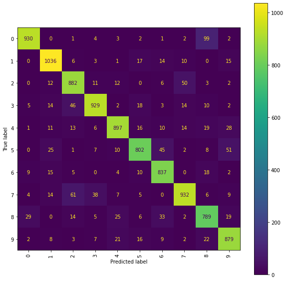
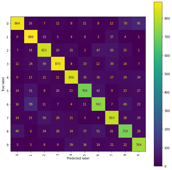
To examine the performance of the best Ridge models we print the confusion matrix and a normalised confusion matrix which highlights only the incorrect classifications.
We first do this for the best Ridge model achieved using the mean and range renormalised paths.
print("The best Ridge model using the mean and range renormalised paths achieved an "
      "accuracy_score of {} on the testing set and corresponds to using the scalefactor {}"
      .format(best_ridge_snmr[2], best_ridge_snmr[0]) )
The best Ridge model using the mean and range renormalised paths achieved an accuracy_score of 0.8931 on the testing set and corresponds to using the scalefactor 4.0
from sklearn.metrics import ConfusionMatrixDisplay
labels = list(range(10))
Ridge Confusion Matrix (snmr)
fig = plt.figure(figsize=(10, 10))
ax = fig.add_subplot(111)
cm_display = ConfusionMatrixDisplay(best_ridge_snmr[3], display_labels=labels).plot(ax=ax,
                                                                                    xticks_rotation="vertical")

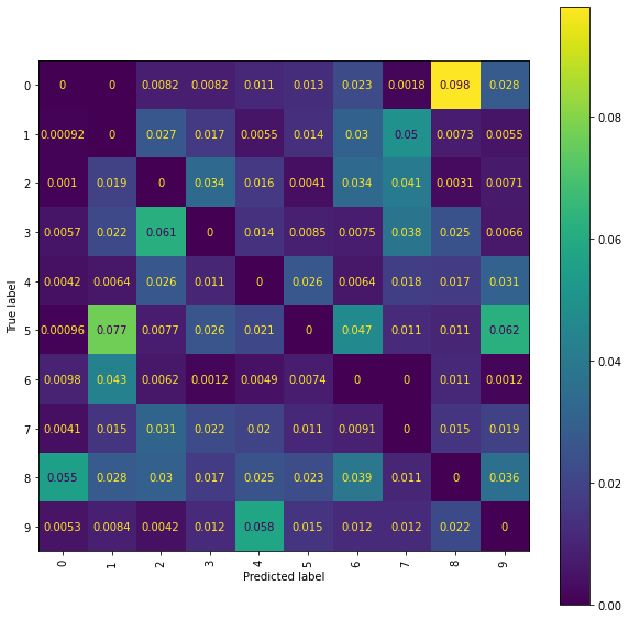
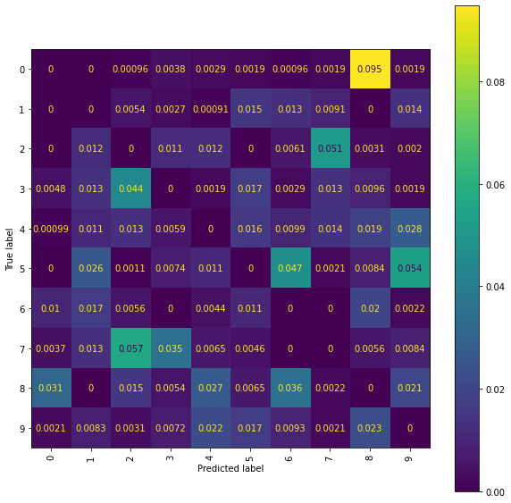
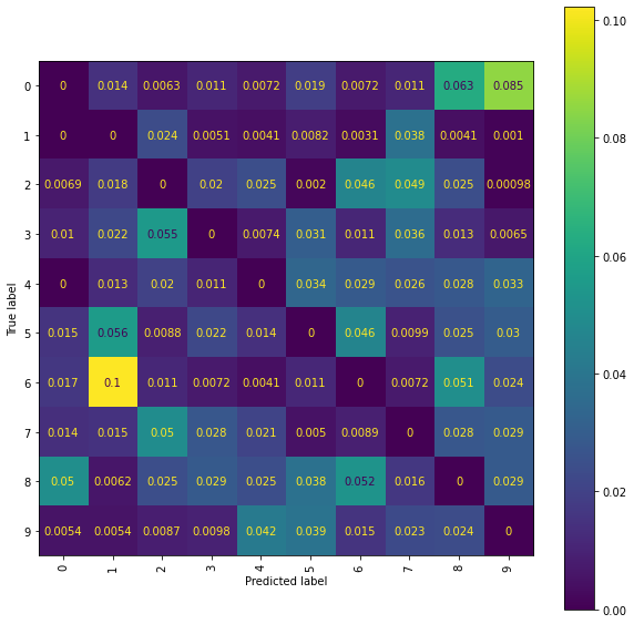
Ridge Normalised Error-Only Confusion Matrix (snmr)
fig = plt.figure(figsize=(10, 10))
ax = fig.add_subplot(111)
cm_display = ConfusionMatrixDisplay(best_ridge_snmr[4], display_labels=labels).plot(ax=ax,
                                                                                    xticks_rotation="vertical")
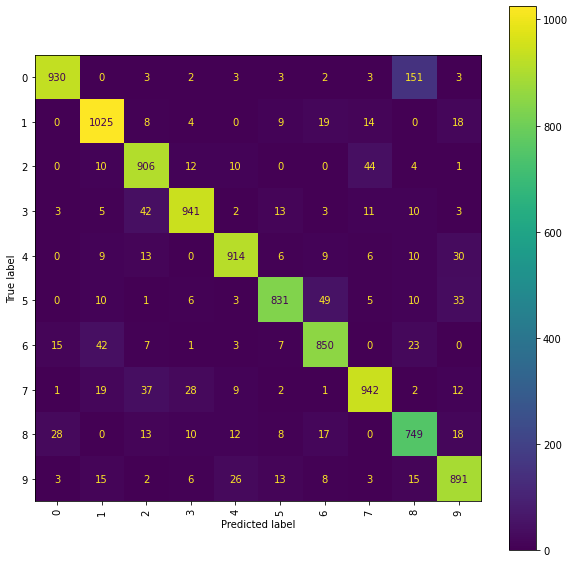
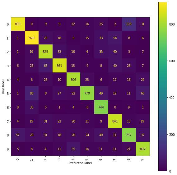
Now we turn our attention to the best Ridge model achieved using the mean and standard deviation renormalised paths.
print("The best Ridge model using the mean and standard deviation renormalised paths achieved an " +
     "accuracy_score of {} on the testing set ".format(best_ridge_snms[2]) +
     "and corresponds to using the scalefactor {}.".format(best_ridge_snms[0]))
The best Ridge model using the mean and standard deviation renormalised paths achieved an accuracy_score of 0.9125 on the testing set and corresponds to using the scalefactor 1.5.
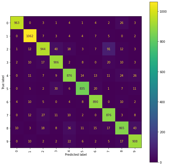
Ridge Confusion Matrix (snms)
fig = plt.figure(figsize=(10, 10))
ax = fig.add_subplot(111)
cm_display = ConfusionMatrixDisplay(best_ridge_snms[3], display_labels=labels).plot(ax=ax,
                                                                                    xticks_rotation="vertical")
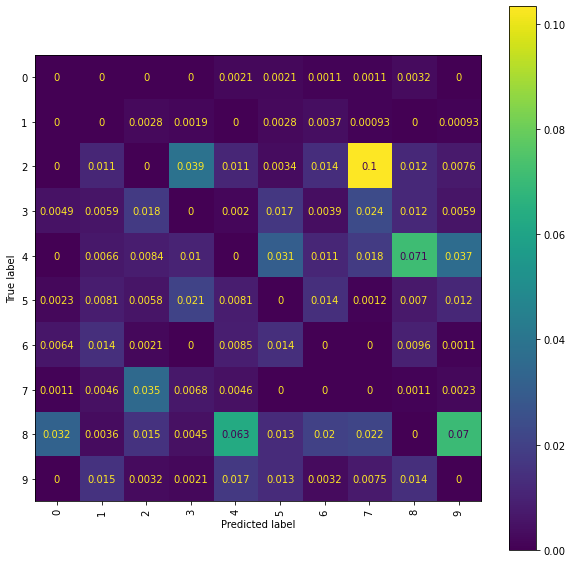
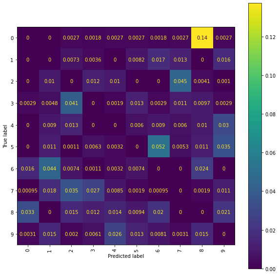
Ridge Normalised Error-Only Confusion Matrix (snms)
fig = plt.figure(figsize=(10, 10))
ax = fig.add_subplot(111)
cm_display = ConfusionMatrixDisplay(best_ridge_snms[4], display_labels=labels).plot(ax=ax,
                                                                                    xticks_rotation="vertical")
The accuracy scores achieved on the testing set are summarised in the following table. In the ‘Sequence Normalisation’ column, snmr means that the signatures were computed from the location sequences normalised to have mean \(0\) and live in \([-1,1]^2\), whilst snms means the signatures were computed from the location sequences normalised to have mean \(0\) and standard deviation \(1\). The model returning the highest accuracy score is highlighted in bold.
Model |
Sequence Normalisation |
Accuracy (%) |
|---|---|---|
Ridge |
snmr |
89.31 |
Ridge |
snms |
91.25 |
An issue is misclassification of \(2\)’s and \(7\)’s, with quite a few \(2\)’s getting incorrectly classified as \(7\)’s. Whilst using higher level signatures may solve this problem it will also be costly, with the number of terms involved in each signature roughly doubling with each new level included. An alternative solution is offered by considering the pen stroke sequences instead; drawing a \(7\) often requires two strokes, whereas drawing a \(2\) only requires a single stroke.
Pen Strokes Sequences
Thus far we have only used the location sequences in \(\mathbb{R}^2\). Now we turn our attention to the pen stroke sequences in \(\mathbb{R}^3\). Rather than use the raw pen stroke sequence, we will first replace each sequence by the sequence of its cumulative sums. That is, the sequence whose \(n^{th}\) entry is the sum of the first \(n\) entries of the original sequence.
The resulting sequence will have its first two components exactly the same as the location sequence, but the additional third component will now count the number of strokes involved (with \(0\) meaning there is only a single stroke, \(1\) meaning there is two strokes, and so on). The signatures of these paths will still capture all the location information as well as additionally capturing information about the number of strokes. As mentioned above, it seems plausible that the number of strokes should help distinguish between a \(2\) and a \(7\).
In effect we are considering an Invisibility Reset-Like transformation of each sequence of locations. We have introduced a new dimension to the sequence and only make this new dimension visible if the number of strokes increases above \(1\).
We start by obtaining the invisibility reset location sequences from the pen stroke sequences by using the ‘inv_reset_like_sum’ function from MNIST_funcs.
help(MNIST_funcs.inv_reset_like_sum)
Help on function inv_reset_like_sum in module MNIST_funcs:

inv_reset_like_sum(stream)
    The input stream is a numpy array. The returned output is a numpy array of
    the same shape, but where the n^th entry in the output is given by the
    component-wise sum of the first n entries in stream.
from MNIST_funcs import inv_reset_like_sum
train_points_ir = Parallel(n_jobs=N_CPU)([delayed(inv_reset_like_sum)(q) for q in train_inputs])
test_points_ir = Parallel(n_jobs=N_CPU)([delayed(inv_reset_like_sum)(q) for q in test_inputs])
Below is an example comparing these new transformed sequences with the original sequences of locations.
train_points[2]
array([[ 5.,  9.],
       [ 5., 10.],
       [ 5., 11.],
       [ 5., 12.],
       [ 5., 13.],
       [ 4., 14.],
       [ 4., 15.],
       [ 5., 16.],
       [ 6., 16.],
       [ 7., 16.],
       [ 8., 16.],
       [ 9., 16.],
       [10., 16.],
       [11., 16.],
       [12., 16.],
       [13., 16.],
       [14., 15.],
       [15., 15.],
       [16., 15.],
       [17., 15.],
       [18., 15.],
       [19., 15.],
       [19., 16.],
       [19., 17.],
       [19., 18.],
       [18., 19.],
       [18., 20.],
       [18., 21.],
       [18., 22.],
       [18., 23.],
       [-1., -1.],
       [19., 14.],
       [20., 13.],
       [20., 12.],
       [20., 11.],
       [21., 10.],
       [21.,  9.],
       [22.,  8.],
       [22.,  7.],
       [22.,  6.]])
train_points_ir[2]
array([[ 5.,  9.,  0.],
       [ 5., 10.,  0.],
       [ 5., 11.,  0.],
       [ 5., 12.,  0.],
       [ 5., 13.,  0.],
       [ 4., 14.,  0.],
       [ 4., 15.,  0.],
       [ 5., 16.,  0.],
       [ 6., 16.,  0.],
       [ 7., 16.,  0.],
       [ 8., 16.,  0.],
       [ 9., 16.,  0.],
       [10., 16.,  0.],
       [11., 16.,  0.],
       [12., 16.,  0.],
       [13., 16.,  0.],
       [14., 15.,  0.],
       [15., 15.,  0.],
       [16., 15.,  0.],
       [17., 15.,  0.],
       [18., 15.,  0.],
       [19., 15.,  0.],
       [19., 16.,  0.],
       [19., 17.,  0.],
       [19., 18.,  0.],
       [18., 19.,  0.],
       [18., 20.,  0.],
       [18., 21.,  0.],
       [18., 22.,  0.],
       [18., 23.,  0.],
       [18., 23.,  1.],
       [19., 14.,  1.],
       [20., 13.,  1.],
       [20., 12.,  1.],
       [20., 11.,  1.],
       [21., 10.,  1.],
       [21.,  9.,  1.],
       [22.,  8.,  1.],
       [22.,  7.,  1.],
       [22.,  6.,  1.]])
Each sequence in train_points_ir and test_points_ir gives rise to a piecewise continuous path in \(\mathbb{R}^3\) via piecewise linear interpolation between the points. Working in dimension \(3\) means that the number of terms in the level \(N\) truncated signature of such a path is now \(\sum_{i=0}^N 3^i = \frac{3^{N+1} - 1}{2}\), meaning that using level \(8\) truncated signatures as before would now involve \(9841\) integral computations for each path.
Since this Notebook is designed for illustration rather than optimal performance, we instead consider level \(5\) truncated signatures of these paths. This limits the number of integral computations involved in calculating the truncated signature of each path to a more reasonable \(364\). Once again, we consider such signatures coming from two different normalisations of these sequences; the first when the sequence components are normalised to have mean \(0\) and live in \([-1,1]\), and the second when the sequence components are normalised to have mean \(0\) and standard deviation \(1\).
SIGNATURE_LEVEL = 5
train_sigs_ir_snmr = Parallel(n_jobs=N_CPU)([delayed(esig.stream2sig)(snmr(train_points_ir[k]), SIGNATURE_LEVEL)
                                             for k in range(len(train_points_ir))])
test_sigs_ir_snmr = Parallel(n_jobs=N_CPU)([delayed(esig.stream2sig)(snmr(test_points_ir[k]), SIGNATURE_LEVEL)
                                            for k in range(len(test_points_ir))])

train_sigs_ir_snms = Parallel(n_jobs=N_CPU)([delayed(esig.stream2sig)(snms(train_points_ir[k]), SIGNATURE_LEVEL)
                                             for k in range(len(train_points_ir))])
test_sigs_ir_snms = Parallel(n_jobs=N_CPU)([delayed(esig.stream2sig)(snms(test_points_ir[k]), SIGNATURE_LEVEL)
                                            for k in range(len(test_points_ir))])
We can now use these new signatures as the feature set for training a classifier.
In the cell below, we use the level \(5\) truncated signatures coming from the transformed location paths in \(\mathbb{R}^3\), renormalised to have mean \(0\) and live in \([-1,1]^3\), and we consider the range of signature scale factors \(r \in \{ 1 , 2 , 3 , 4 \}\) as before.
ridge_results_ir_snmr, ridge_best_result_ir_snmr = ridge_scale_learn(E, 3, SIGNATURE_LEVEL, train_sigs_ir_snmr,
                                                                     train_targets,
                                                                     reg=[np.array((0.01,0.1,1.0,10.0))],
                                                                     cpu_number_one=N_CPU//4 ,
                                                                     cpu_number_two = N_CPU//4)
In the cell below, we use the level \(5\) truncated signatures coming from the transformed location paths in \(\mathbb{R}^3\), renormalised to have mean \(0\) and standard deviation \(1\), and we consider the range of signature scale factors \(r \in \{ 0.5 , 1 , 1.5 , 2 \}\) as before.
ridge_results_ir_snms, ridge_best_result_ir_snms = ridge_scale_learn(EB, 3, SIGNATURE_LEVEL,
                                                                     train_sigs_ir_snms,
                                                                     train_targets,
                                                                     reg=[np.array((0.01,0.1,1.0,10.0))],
                                                                     cpu_number_one=N_CPU//4 ,
                                                                     cpu_number_two = N_CPU//4)
Testing Set Performance - Transformed Location Sequences
We now use the ‘model_performance’ function to see how well our models learnt using the transformed location sequences perform on the testing set.
best_ridge_ir_snmr = model_performance(ridge_best_result_ir_snmr, 3, SIGNATURE_LEVEL, test_sigs_ir_snmr,
                                       test_targets,
                                       cpu_number=N_CPU)
best_ridge_ir_snms = model_performance(ridge_best_result_ir_snms, 3, SIGNATURE_LEVEL,test_sigs_ir_snms,
                                       test_targets,
                                       cpu_number=N_CPU)
Ridge Classifier Results
To examine the performance of the best Ridge models we print the confusion matrix and a normalised confusion matrix which highlights only the incorrect classifications.
We first do this for the best Ridge model achieved using the mean and range renormalised paths.
print("The best Ridge model using the mean and range renormalised paths "
      "(coming from the transformed location sequences) achieved an "
      "accuracy_score of {} on the testing set "
      "and corresponds to using the scalefactor {}.".format(best_ridge_ir_snmr[2], best_ridge_ir_snmr[0]))
The best Ridge model using the mean and range renormalised paths (coming from the transformed location sequences) achieved an accuracy_score of 0.8913 on the testing set and corresponds to using the scalefactor 2.0.
Ridge Confusion Matrix (ir snmr)
fig = plt.figure(figsize=(10, 10))
ax = fig.add_subplot(111)
cm_display = ConfusionMatrixDisplay(best_ridge_ir_snmr[3],
                                    display_labels=labels).plot(ax=ax, xticks_rotation="vertical")
Ridge Normalised Error-Only Confusion Matrix (ir snmr)
fig = plt.figure(figsize=(10, 10))
ax = fig.add_subplot(111)
cm_display = ConfusionMatrixDisplay(best_ridge_ir_snmr[4],
                                    display_labels=labels).plot(ax=ax, xticks_rotation="vertical")
Now we turn our attention to the best Ridge model achieved using the mean and standard deviation renormalised paths.
print("The best Ridge model using the mean and standard deviation renormalised paths "
      "(coming from the transformed location sequences) achieved an "
      "accuracy_score of {} on the testing set "
      "and corresponds to using the scalefactor {}.".format(best_ridge_ir_snms[2], best_ridge_ir_snms[0]))
The best Ridge model using the mean and standard deviation renormalised paths (coming from the transformed location sequences) achieved an accuracy_score of 0.8979 on the testing set and corresponds to using the scalefactor 2.0.
Ridge Confusion matrix (ir snms)
fig = plt.figure(figsize=(10, 10))
ax = fig.add_subplot(111)
cm_display = ConfusionMatrixDisplay(best_ridge_ir_snms[3],
                                    display_labels=labels).plot(ax=ax, xticks_rotation="vertical")
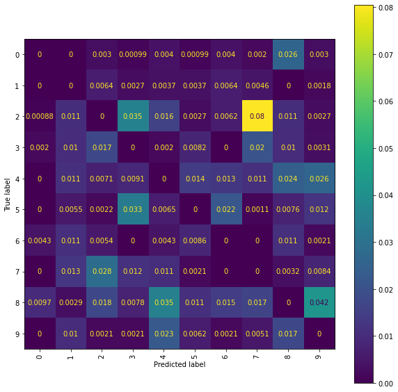
Ridge Normalised Error-Only Confusion Matrix (ir snms)
fig = plt.figure(figsize=(10, 10))
ax = fig.add_subplot(111)
cm_display = ConfusionMatrixDisplay(best_ridge_ir_snms[4],
                                    display_labels=labels).plot(ax=ax, xticks_rotation="vertical")
Using transformed location sequences has had a positive impact on one part of the 2/7 classification, with an examination of the confusion matrices showing that the number of \(2\)s incorrectly classified as a \(7\) has been reduced compared to the results obtained using the original location sequences. However, in all but one of the models, the number of \(7\)’s incorrectly classified as a \(2\) has increased, suggesting that the deeper level signature terms were important for this decision. It is also noticeable that using a lower truncation level has deteriorated the performance of some models on other particular comparisons (for example, the RFC models are both now incorrectly classifying more \(0\)s as \(8\)s than previously).
It is likely that truncating at level \(5\) has lost valuable information that was previously useful. The feature set obtained from the transformed sequences consists only of \(364\) terms compared to the \(511\) obtained from the original location sequences. Depending on the hardware available, the reader may like to try using higher truncation levels with the transformed location sequences. Since this Notebook is designed mainly for illustration we do not do so here.
Unsupervised Learning
We now briefly explore what we can achieve without making use of the labels, i.e. without using the lists train_targets and test_targets. Without access to labels for the data, we will try a clustering approach. That is, to try and split the data into similar groups with the idea that instances belonging to the same group should represent the same digit, even if we do not know what digit that is.
Naively, we may hope that searching for \(10\) groups will give good results since there are \(10\) distinct digits to recognise, i.e. the \(10\) digits \(\{0,1,2,3,4,5,6,7,8,9\}\). We first try this using the Scikit-Learn KMeans model (https://scikit-learn.org/stable/modules/generated/sklearn.cluster.KMeans.html) searching for \(10\) clusters. For this we use the ‘kmeans_fit’ function from MNIST_funcs.
help(MNIST_funcs.kmeans_fit)
Help on function kmeans_fit in module MNIST_funcs:

kmeans_fit(a, data)
    a is an integer in [2, len(data) - 1] and data is a list of float-valued
    numpy arrays.

    The returned output is a KMeans cluster model, with n_clusters = a, fitted
    to data.
We consider signatures coming from both the original location sequences and the transformed sequences. We also consider both the mean and range normalised sequences and the mean and standard deviation normalised sequences for each set of signatures.
from MNIST_funcs import kmeans_fit
N_CLUSTERS = 10
Naive_cluster_snmr = kmeans_fit(N_CLUSTERS, train_sigs_snmr)
Naive_cluster_snms = kmeans_fit(N_CLUSTERS, train_sigs_snms)
Naive_cluster_ir_snmr = kmeans_fit(N_CLUSTERS, train_sigs_ir_snmr)
Naive_cluster_ir_snms = kmeans_fit(N_CLUSTERS, train_sigs_ir_snms)
We evaluate the performance via the silhouette_score (https://scikit-learn.org/stable/modules/generated/sklearn.metrics.silhouette_score.html) of each model. This involves using each model to first predict the labels for each instance in the respective collections of signatures.
from sklearn.metrics import silhouette_score
A = silhouette_score(train_sigs_snmr, Naive_cluster_snmr.labels_)
B = silhouette_score(train_sigs_snms, Naive_cluster_snms.labels_ )
C = silhouette_score(train_sigs_ir_snmr, Naive_cluster_ir_snmr.labels_)
D = silhouette_score(train_sigs_ir_snms, Naive_cluster_ir_snms.labels_)
A,B,C,D
(0.3423609233626098,
 0.2473760853401116,
 0.28616143525417015,
 0.20279287613045088)
These scores are not particularly good. This isn’t that surprising; it is easy to imagine two figure \(4\)’s that bare little similarity to one and other, for example. Moreover, as we have seen previously, there are many figure \(2\)’s that are quite similar to \(7\)’s, and vice versa. The issue is that \(x\) being a digit \(a\) does not guarantee that - \(x\) very close to all other instances of the digit \(a\), and that - \(x\) is not close to any instance of a digit that is not \(a\)
Semi-Supervised Learning
The starting point is noting that each fitted KMeans model returns a centroid element for each cluster it finds. For example, if we look at the Naive_cluster_snmr model that split the train_sigs_snmr into \(10\) clusters (which subsequently turned out to be the best number of clusters in terms of silhouette_score), then the centroid elements are displayed via the cell below.
Naive_cluster_snmr.cluster_centers_
array([[ 1.00000000e+00,  1.94641871e-01,  2.56122612e-03, ...,
         7.42651064e-06, -3.28060199e-06,  3.68675850e-08],
       [ 1.00000000e+00, -1.58339423e-02,  6.98912294e-02, ...,
         2.47294787e-04, -4.17336864e-05,  1.64097507e-08],
       [ 1.00000000e+00, -9.21419107e-01,  9.60767338e-01, ...,
         2.57751418e-06, -4.71207138e-05,  2.06990909e-05],
       ...,
       [ 1.00000000e+00,  9.16349602e-01,  9.15180493e-01, ...,
        -3.10950556e-06,  5.13662764e-05,  1.68285371e-05],
       [ 1.00000000e+00,  9.17817383e-01, -8.40123738e-01, ...,
         2.96427181e-05, -6.11327797e-05,  1.07901653e-05],
       [ 1.00000000e+00,  5.61114765e-02, -5.58955107e-01, ...,
        -3.03212495e-04,  1.06641392e-04,  9.95886107e-07]])
We can use the centroid elements found during the KMeans clustering to develop a semi-supervised learning approach as follows: - Apply KMeans clustering algorithm to split the signatures into clusters - Assign each clusters centroid element its corresponding label - Propagate this label out to the closest \(a\)% of elements in each cluster where \(a\) can be chosen by us - Use the elements that are given this label as the training set for the various supervised learning models we considered previously - Evaluate the performance of the trained models using the untouched testing set
A priori, this appears to require far fewer labelled training instances. For example, the Naive_cluster_snmr model returns \(10\) clusters, and so we only need to know the labels associated to \(10\) of the \(60000\) training instances. But, the centroid elements are determined during the clustering, and so it is only afterwards that we know which \(10\) labels we need. Beforehand, the centroid elements could be any of the \(60000\) training instances, meaning we do need to know the labels for all training instances to ensure we can assign the chosen centroid elements there labels.
However, since the subsequent learning is only carried out on labelled data obtained by propagating the centroid labels to the nearest \(a\)% of their clusters, we can expect the learning to be faster than when we used the full \(60000\) training instances (assuming that \(a < 100\), of course).
To carry out this strategy we use the ‘kmeans_percentile_propagate’ function from MNIST_funcs.
help(MNIST_funcs.kmeans_percentile_propagate)
Help on function kmeans_percentile_propagate in module MNIST_funcs:

kmeans_percentile_propagate(cluster_num, percent, data, labels)
    cluster_num is an integer in [2, len(data)-1], percent is a float in
    [0,100], data is a list of float-valued numpy arrays and labels is a list,
    of same length as data, of integers.

    A KMeans model with cluster_num clusters is used to fit_transform data.

    A representative centroid element from each cluster is assigned its
    corresponding label from the labels list.

    This label is then propagated to the percent% of the instances in the
    cluster that are closest to the clusters centroid.

    The returned output is a list of these chosen instances and a list of the
    corresponding labels for these instances.
We apply ‘kmeans_percentile_propagate’ to the four collections of training signatures that we have previously used with the choice of percent \(=10\).
from MNIST_funcs import kmeans_percentile_propagate
P = 10

train_sigs_snmr_P ,train_targets_snmr_P = kmeans_percentile_propagate(cluster_num=10, percent=P,
                                                                      data=train_sigs_snmr,
                                                                      labels=train_targets)

train_sigs_snms_P ,train_targets_snms_P = kmeans_percentile_propagate(cluster_num=15, percent=P,
                                                                      data=train_sigs_snms,
                                                                      labels=train_targets)

train_sigs_ir_snmr_P ,train_targets_ir_snmr_P = kmeans_percentile_propagate(cluster_num=20,
                                                                            percent=P,
                                                                            data=train_sigs_ir_snmr,
                                                                            labels=train_targets)

train_sigs_ir_snms_P ,train_targets_ir_snms_P = kmeans_percentile_propagate(cluster_num=50,
                                                                            percent=P,
                                                                            data=train_sigs_ir_snms,
                                                                            labels=train_targets)
Level 8 Truncated Signatures of Paths from Location Sequences with Mean and Range Normalisation
We train a Ridge model on the propagated set of signatures arising from the level 8 truncated signatures of the paths from the mean and range normalised location sequences.
SIGNATURE_LEVEL = 8

ridge_results_snmr_P, ridge_best_result_snmr_P = ridge_scale_learn(E, 2, SIGNATURE_LEVEL,
                                                                   train_sigs_snmr_P,
                                                                   train_targets_snmr_P,
                                                                   reg=[np.array((0.01,0.1,1.0,10.0))],
                                                                   cpu_number_one=N_CPU//4 ,
                                                                   cpu_number_two = N_CPU//4)
Now we examine the performance of the best trained models of each type on the testing set.
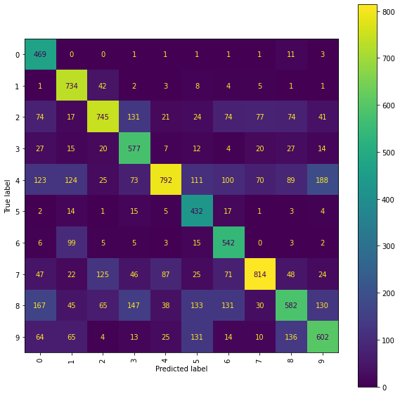
best_ridge_snmr_P = model_performance(ridge_best_result_snmr_P, 2, SIGNATURE_LEVEL, test_sigs_snmr,
                                      test_targets,cpu_number=N_CPU)
print("The best Ridge model achieves an accuracy_score of {} "
      "using a scalefactor of {}.".format(best_ridge_snmr_P[2], best_ridge_snmr_P[0]))
The best Ridge model achieves an accuracy_score of 0.6289 using a scalefactor of 4.0.
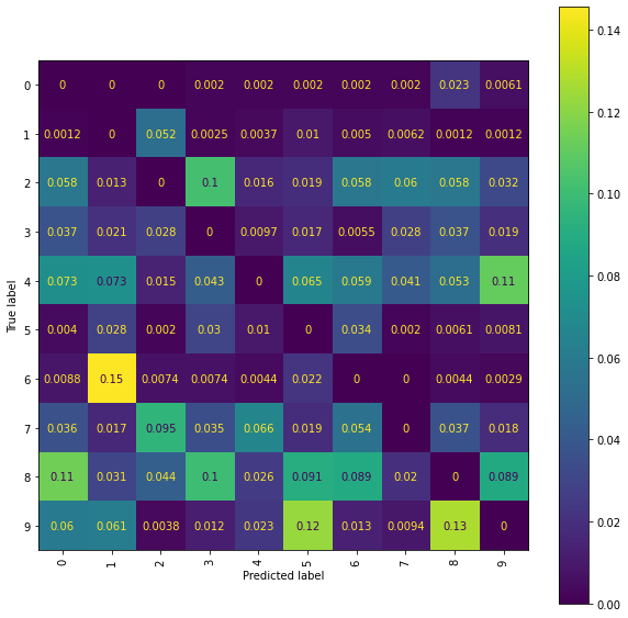
Once again, we carry out a more detailed examination by looking at the confusion matrices and the normalised confusion matrices focusing only on the incorrect classifications.
Ridge Confusion Matrix
fig = plt.figure(figsize=(10, 10))
ax = fig.add_subplot(111)
cm_display = ConfusionMatrixDisplay(best_ridge_snmr_P[3],
                                    display_labels=labels).plot(ax=ax, xticks_rotation="vertical")
Ridge Normalised Error-Only Confusion Matrix
fig = plt.figure(figsize=(10, 10))
ax = fig.add_subplot(111)
cm_display = ConfusionMatrixDisplay(best_ridge_snmr_P[4],
                                    display_labels=labels).plot(ax=ax, xticks_rotation="vertical")
Level 8 Truncated Signatures of Paths from Location Sequences with Mean and Standard Deviation Normalisation
We train a Ridge model on the propagated set of signatures arising from the level 8 truncated signatures of the paths from the mean and standard deviation normalised location sequences.
ridge_results_snms_P, ridge_best_result_snms_P = ridge_scale_learn(EB, 2, SIGNATURE_LEVEL,
                                                                   train_sigs_snms_P,
                                                                   train_targets_snms_P,
                                                                   reg=[np.array((0.01,0.1,1.0,10.0))],
                                                                   cpu_number_one=N_CPU//4,
                                                                   cpu_number_two=N_CPU//4)
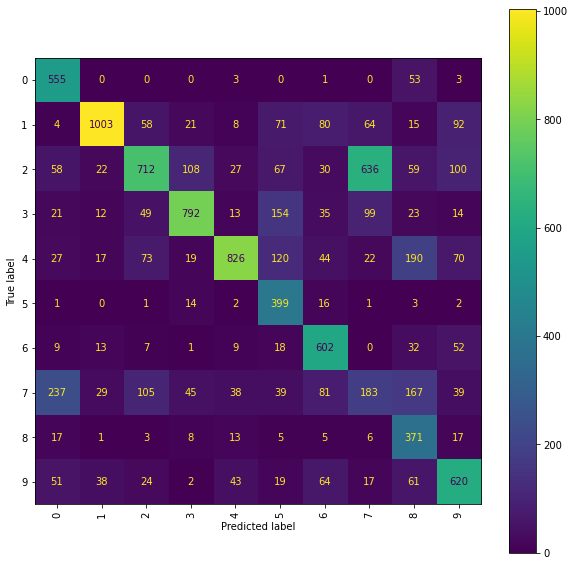
Now we examine the performance of the best models of each type on the testing set.
best_ridge_snms_P = model_performance(ridge_best_result_snms_P, 2, SIGNATURE_LEVEL,
                                      test_sigs_snms,test_targets,cpu_number=N_CPU)

print("The best Ridge model achieves an accuracy_score of {} "
      "using a scalefactor of {}.".format(best_ridge_snms_P[2], best_ridge_snms_P[0]))
The best Ridge model achieves an accuracy_score of 0.6063 using a scalefactor of 2.0.
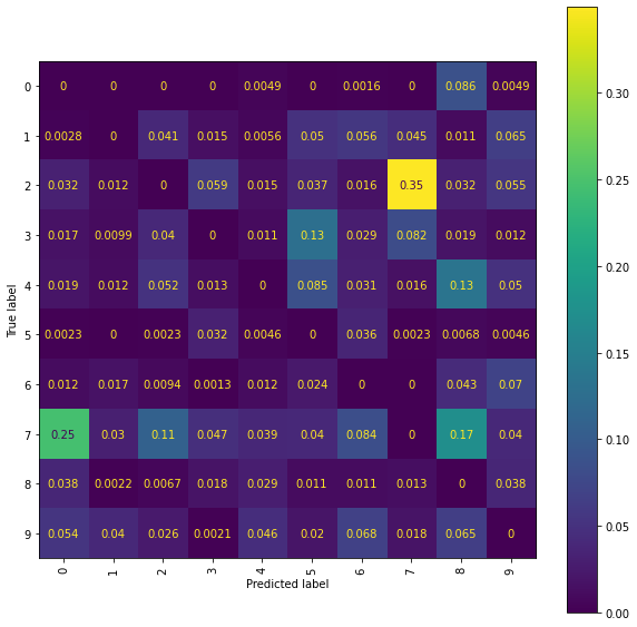
A more detailed examination of the performance can be carried out from the confusion matrices and the normalised error-only confusion matrices.
Ridge Confusion Matrix
fig = plt.figure(figsize=(10, 10))
ax = fig.add_subplot(111)
cm_display = ConfusionMatrixDisplay(best_ridge_snms_P[3],
                                    display_labels=labels).plot(ax=ax, xticks_rotation="vertical")
Ridge Normalised Error-Only Confusion Matrix
fig = plt.figure(figsize=(10, 10))
ax = fig.add_subplot(111)
cm_display = ConfusionMatrixDisplay(best_ridge_snms_P[4],
                                    display_labels=labels).plot(ax=ax, xticks_rotation="vertical")
Level 5 Truncated Signatures of Paths from Transformed Location Sequences with Mean and Range Normalisation
We train a Ridge model on the propagated set of signatures arising as the level 5 truncated signatures of the paths from the mean and range normalised transformed location sequences.
SIGNATURE_LEVEL = 5

ridge_results_ir_snmr_P, ridge_best_result_ir_snmr_P = ridge_scale_learn(E,3, SIGNATURE_LEVEL,
                                                                         train_sigs_ir_snmr_P,
                                                                         train_targets_ir_snmr_P,
                                                                         reg=[np.array((0.01,0.1,1.0,10.0))],
                                                                         cpu_number_one=N_CPU//4,
                                                                         cpu_number_two = N_CPU//4)
Now examine the performance of the best models of each type on the testing set.
best_ridge_ir_snmr_P = model_performance(ridge_best_result_ir_snmr_P, 3, SIGNATURE_LEVEL,
                                         test_sigs_ir_snmr, test_targets,cpu_number=N_CPU)

print("The best Ridge model achieves an accuracy_score of {} "
      "using a scalefactor of {}.".format(best_ridge_ir_snmr_P[2], best_ridge_ir_snmr_P[0]))
The best Ridge model achieves an accuracy_score of 0.8009 using a scalefactor of 4.0.
Again a more detailed examination of the performances can be achieved by viewing the confusion matrices and the normalised error-only confusion matrices.
Ridge Confusion Matrix
fig = plt.figure(figsize=(10, 10))
ax = fig.add_subplot(111)
cm_display = ConfusionMatrixDisplay(best_ridge_ir_snmr_P[3],
                                    display_labels=labels).plot(ax=ax, xticks_rotation="vertical")
Ridge Normalised Error-Only Confusion Matrix
fig = plt.figure(figsize=(10, 10))
ax = fig.add_subplot(111)
cm_display = ConfusionMatrixDisplay(best_ridge_ir_snmr_P[4],
                                    display_labels=labels).plot(ax=ax, xticks_rotation="vertical")
Level 5 Truncated Signatures of Paths from Transformed Location Sequences with Mean and Standard Deviation Normalisation
We train a Ridge model on the propagated set of signatures arising as the level 5 truncated signatures of the paths from the mean and standard deviation normalised transformed location sequences.
ridge_results_ir_snms_P, ridge_best_result_ir_snms_P = ridge_scale_learn(EB, 3, SIGNATURE_LEVEL,
                                                                         train_sigs_ir_snms_P,
                                                                         train_targets_ir_snms_P,
                                                                         reg=[np.array((0.01,0.1,1.0,10.0))],
                                                                         cpu_number_one=N_CPU//4,
                                                                         cpu_number_two = N_CPU//4)
Now examine the performance of the best models of each type on the test set.
best_ridge_ir_snms_P = model_performance(ridge_best_result_ir_snms_P, 3, SIGNATURE_LEVEL,
                                         test_sigs_ir_snms,test_targets,cpu_number=N_CPU)

print("The best Ridge model achieves an accuracy_score of {} "
      "using a scalefactor of {}.".format(best_ridge_ir_snms_P[2], best_ridge_ir_snms_P[0]))
The best Ridge model achieves an accuracy_score of 0.8224 using a scalefactor of 2.0.
Again a more detailed examination of the performance may be obtained by viewing the confusion matrices and the normalised error-only confusion matrices.
Ridge Confusion Matrix
fig = plt.figure(figsize=(10, 10))
ax = fig.add_subplot(111)
cm_display = ConfusionMatrixDisplay(best_ridge_ir_snms_P[3],
                                    display_labels=labels).plot(ax=ax, xticks_rotation="vertical")
Ridge Normalised Error-Only Confusion Matrix
fig = plt.figure(figsize=(10, 10))
ax = fig.add_subplot(111)
cm_display = ConfusionMatrixDisplay(best_ridge_ir_snms_P[4],
                                    display_labels=labels).plot(ax=ax, xticks_rotation="vertical")