Controlled Neural Differential Equations - Time Series Classification
This notebook is based on the examples from the torchcde package by
Kidger and Morrill which can be found at
https://github.com/patrick-kidger/torchcde. Further information about
the techniques described in this notebook can be found
Kidger, P., Morrill, J., Foster, J. and Lyons, T., 2020. Neural controlled differential equations for irregular time series. arXiv preprint arXiv:2005.08926.
Morrill, J., Kidger, P., Yang, L. and Lyons, T., 2021. Neural Controlled Differential Equations for Online Prediction Tasks. arXiv preprint arXiv:2106.11028.
Kidger, P., Foster, J., Li, X., Oberhauser, H. and Lyons, T., 2021. Neural sdes as infinite-dimensional gans. arXiv preprint arXiv:2102.03657.
In this notebook we explore the classification of time series data using controlled neural differential equations.
Set up the notebook
Install dependencies
This notebook requires PyTorch and the torchcde package. The
dependencies are listed in the requirements.txt file. They can be
installed using the following command.
import sys
!{sys.executable} -m pip uninstall -y enum34
!{sys.executable} -m pip install -r requirements.txt
Import the necessary packages
import math
import numpy as np
import torch
import torchcde
import matplotlib.pyplot as plt
Also set some parameters that can be changed when experimenting with the method.
HIDDEN_LAYER_WIDTH = 64  # This is the width of the hidden layer of the neural network
NUM_EPOCHS = 10  # This is the number of training iterations we will use later
BATCH_SIZE = 32  # Size of batch used in the training process
Set up the helper classes
A controlled differential equation (CDE) model looks like
where \(X\) is your data and \(f_\theta\) is a neural network.
So the first thing we need to do is define such an \(f_\theta\).
That’s what this CDEFunc class does. Here we’ve built a small
single-hidden-layer neural network, whose hidden layer is of width
HIDDEN_LAYER_WIDTH set above.
class CDEFunc(torch.nn.Module):
    def __init__(self, input_channels, hidden_channels):
        ######################
        # input_channels is the number of input channels in the data X. (Determined by the data.)
        # hidden_channels is the number of channels for z_t. (Determined by you!)
        ######################
        super(CDEFunc, self).__init__()
        self.input_channels = input_channels
        self.hidden_channels = hidden_channels

        self.linear1 = torch.nn.Linear(hidden_channels, HIDDEN_LAYER_WIDTH)
        self.linear2 = torch.nn.Linear(HIDDEN_LAYER_WIDTH, input_channels * hidden_channels)

    ######################
    # For most purposes the t argument can probably be ignored; unless you want your CDE to behave differently at
    # different times, which would be unusual. But it's there if you need it!
    ######################
    def forward(self, t, z):
        # z has shape (batch, hidden_channels)
        z = self.linear1(z)
        z = z.relu()
        z = self.linear2(z)
        ######################
        # Easy-to-forget gotcha: Best results tend to be obtained by adding a final tanh nonlinearity.
        ######################
        z = z.tanh()
        ######################
        # Ignoring the batch dimension, the shape of the output tensor must be a matrix,
        # because we need it to represent a linear map from R^input_channels to R^hidden_channels.
        ######################
        z = z.view(z.size(0), self.hidden_channels, self.input_channels)
        return z
Next, we need to package CDEFunc up into a model that computes the integral.
class NeuralCDE(torch.nn.Module):
    def __init__(self, input_channels, hidden_channels, output_channels, interpolation="cubic"):
        super(NeuralCDE, self).__init__()

        self.func = CDEFunc(input_channels, hidden_channels)
        self.initial = torch.nn.Linear(input_channels, hidden_channels)
        self.readout = torch.nn.Linear(hidden_channels, output_channels)
        self.interpolation = interpolation

    def forward(self, coeffs):
        if self.interpolation == 'cubic':
            X = torchcde.NaturalCubicSpline(coeffs)
        elif self.interpolation == 'linear':
            X = torchcde.LinearInterpolation(coeffs)
        else:
            raise ValueError("Only 'linear' and 'cubic' interpolation methods are implemented.")

        ######################
        # Easy to forget gotcha: Initial hidden state should be a function of the first observation.
        ######################
        X0 = X.evaluate(X.interval[0])
        z0 = self.initial(X0)

        ######################
        # Actually solve the CDE.
        ######################
        z_T = torchcde.cdeint(X=X,
                              z0=z0,
                              func=self.func,
                              t=X.interval)

        ######################
        # Both the initial value and the terminal value are returned from cdeint; extract just the terminal value,
        # and then apply a linear map.
        ######################
        z_T = z_T[:, 1]
        pred_y = self.readout(z_T)
        return pred_y
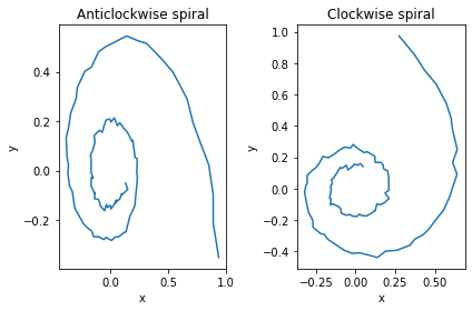
Now we need some data. Here we have a simple example which generates some spirals, some going clockwise, some going anticlockwise.
def get_data(num_timepoints=100):
    """
    Generate time series data with `num_timepoints` data points
    """
    t = torch.linspace(0., 4 * math.pi, num_timepoints)

    start = torch.rand(HIDDEN_LAYER_WIDTH) * 2 * math.pi
    x_pos = torch.cos(start.unsqueeze(1) + t.unsqueeze(0)) / (1 + 0.5 * t)
    x_pos[:HIDDEN_LAYER_WIDTH//2] *= -1
    y_pos = torch.sin(start.unsqueeze(1) + t.unsqueeze(0)) / (1 + 0.5 * t)
    x_pos += 0.01 * torch.randn_like(x_pos)
    y_pos += 0.01 * torch.randn_like(y_pos)
    ######################
    # Easy to forget gotcha: time should be included as a channel; Neural CDEs need to be explicitly told the
    # rate at which time passes. Here, we have a regularly sampled dataset, so appending time is pretty simple.
    ######################
    X = torch.stack([t.unsqueeze(0).repeat(HIDDEN_LAYER_WIDTH, 1), x_pos, y_pos], dim=2)
    y = torch.zeros(HIDDEN_LAYER_WIDTH)
    y[:HIDDEN_LAYER_WIDTH//2] = 1

    perm = torch.randperm(HIDDEN_LAYER_WIDTH)
    X = X[perm]
    y = y[perm]

    ######################
    # X is a tensor of observations, of shape (batch=128, sequence=100, channels=3)
    # y is a tensor of labels, of shape (batch=128,), either 0 or 1 corresponding to anticlockwise or clockwise respectively.
    ######################
    return X, y
Getting the training data
Now we use the get_data function we just defined to create a set of
data to train the model.
train_X, train_y = get_data()
To illustrate the kind of data, we plot examples of the anticlockwise and clockwise spirals from this training set. The radius of the spiral decreases as time progresses.
fig, (ax1, ax2) = plt.subplots(1, 2, tight_layout=True)
idx, = np.where(train_y == 0)
ax1.plot(train_X[idx[0], :, 1], train_X[idx[0], :, 2])
ax1.set_title("Anticlockwise spiral")
ax1.set_xlabel("x")
ax1.set_ylabel("y")

idx, = np.where(train_y == 1)
ax2.plot(train_X[idx[0], :, 1], train_X[idx[0], :, 2])
ax2.set_title("Clockwise spiral")
ax2.set_xlabel("x")
ax2.set_ylabel("y")
plt.show()
input_channels=3 because we have both the horizontal and vertical position of a point in the spiral, and time. hidden_channels=8 is the number of hidden channels for the evolving \(z_t\), which we get to choose. output_channels=1 because we’re doing binary classification.
model = NeuralCDE(input_channels=3, hidden_channels=8, output_channels=1)
optimizer = torch.optim.Adam(model.parameters())
Now we turn our dataset into a continuous path. We do this here via
natural cubic spline interpolation. The resulting train_coeffs is a
tensor describing the path. For most problems, it’s probably easiest to
save this tensor and treat it as the dataset.
train_coeffs = torchcde.natural_cubic_coeffs(train_X)
train_dataset = torch.utils.data.TensorDataset(train_coeffs, train_y)
train_dataloader = torch.utils.data.DataLoader(train_dataset, batch_size=BATCH_SIZE)

for epoch in range(NUM_EPOCHS):
    for batch in train_dataloader:
        batch_coeffs, batch_y = batch
        pred_y = model(batch_coeffs).squeeze(-1)
        loss = torch.nn.functional.binary_cross_entropy_with_logits(pred_y, batch_y)
        loss.backward()
        optimizer.step()
        optimizer.zero_grad()
    print('Epoch: {:2d}   Training loss: {}'.format(epoch, loss.item()))
Epoch:  0   Training loss: 0.7206246852874756
Epoch:  1   Training loss: 0.6758381724357605
Epoch:  2   Training loss: 0.6444145441055298
Epoch:  3   Training loss: 0.6178776025772095
Epoch:  4   Training loss: 0.5846209526062012
Epoch:  5   Training loss: 0.5368350744247437
Epoch:  6   Training loss: 0.48740214109420776
Epoch:  7   Training loss: 0.4454191327095032
Epoch:  8   Training loss: 0.40035274624824524
Epoch:  9   Training loss: 0.35087674856185913
Validating the model
Now we need to validate the model that we have trained. First we create some new data using the same function as before. Then we proceed as before, fitting cubic splines and evaluating the newly trained model on these data.
test_X, test_y = get_data()

test_coeffs = torchcde.natural_cubic_coeffs(test_X)
pred_y = model(test_coeffs).squeeze(-1)
binary_prediction = (torch.sigmoid(pred_y) > 0.5).to(test_y.dtype)
prediction_matches = (binary_prediction == test_y).to(test_y.dtype)
proportion_correct = prediction_matches.sum() / test_y.size(0)
print('Test Accuracy: {}'.format(proportion_correct))
Test Accuracy: 0.984375